Markov Chains Used in Stock Index Forecast

I shortly introduced via a simple weather prediction model the use of Markov chains and respectively Python implementation. Here we will have a look at a stock index – I take the S&P 500 index for the period Aug 5, 2014 to Aug 5, 2015 (252 daily returns) as an example.

First we calculate daily returns and decide on three states of the daily changes – decrease (coded as ‘1’), neutral (coded as ‘2’) and increase (coded as ‘3’). Then we calculate 9 states (resp. probabilities based on historical figures):

(i)                  yesterday index decreased and today  is down as well (coded as ‘11’)

(ii)                yesterday index decreased but today is neutral (coded as ‘12’)

(iii)               yesterday index decreased but today is up (coded as ‘13’)

(iv)              yesterday index was neutral but today is down (coded as ‘21’)

(v)                yesterday index was neutral and today is neutral too (coded as ‘22’)

(vi)              yesterday index was neutral but today is up (coded as ‘23’)

(vii)             yesterday index increased but today is down (coded as ‘31’)

(viii)           yesterday index increased but today is neutral (coded as ‘32’)

(ix)              yesterday index increased and today is up as well (coded as ‘33’)

The algorithm I follow is as follows: (1) count all daily decreases, neutral and increases in index values (i.e. index returns over 1-day period), then (2) count all cases within the nine states (as stated above) – from prior day decrease to current day decrease, from prior day decrease to current day increase and so on and finally (3) calculating the probabilities is straightforward: divide state coded as ‘11’ by total number of daily decreases, divide state coded as ‘12’ by total number of daily decreases, divide state coded as ‘21’ by total number of daily increases and divide state coded as ‘22’ by total number of daily increases and so on.

For instance:

	Counts
Daily decreases (state '1')	121
Daily neutral (state '2')	6
Daily increases (state ‘3’)	125
	Counts	Probabilities
State ‘11’	57	0.47
State ‘12’	1	0.01
State ‘13’	63	0.52
State '21'	3	0.5
State '22'	0	0
State '23'	3	0.5
State '31'	61	0.49
State '31'	4	0.04
State '33'	59	0.47

To From	Decrease (‘1’)	Neutral (‘2’)	Increase (‘3’)
Decrease (‘1’)	0.47 (‘11’)	0.01 (‘12’)	0.52 (‘13’)
Neutral (‘2’)	0.5 (‘21’)	0 (‘22’)	0.5 (‘23’)
Increase (‘3’)	0.49 (‘31’)	0.04  (‘32’)	0.47 (‘33’)

For S&P 500 example there is 47% probability of decrease today given yesterday index decreased and 47% probability of increase today given increased yesterday. Quite fair!

Solving for the steady state probabilities (as explained here: http://elenamarinova.blogspot.com/2015/06/markov-chains-in-python-simple-weather.html) 49% of the days the index will increase and 48% of the days the index will experience a decrease over the prior day. The steady state is already independent on the current state, this is the memoryless property of the process.

(1) transition=np.array([[0.47, 0.01, 0.52],[0.5, 0.00, 0.5], [0.49, 0.04,0.47]])
initial=np.array([0,0,1]) #today is increase
Result: [decrease, neutral, increase]
[ 0.49 0.04 0.47]

[ 0.4806  0.0237  0.4957]
[ 0.480625  0.024634  0.494741]
[ 0.48063384  0.02459589  0.49477027]
[ 0.48063328  0.02459715  0.49476957]
[ 0.48063331  0.02459712  0.49476958]

(2) transition=np.array([[0.47, 0.01, 0.52],[0.5, 0.00, 0.5], [0.49, 0.04,0.47]])

initial=np.array([1,0,0]) #today is decrease

Result: [decrease, neutral, increase]
[ 0.47  0.01  0.52]
[ 0.4807  0.0255  0.4938]
[ 0.480641  0.024559  0.4948  ]
[ 0.48063277  0.02459841  0.49476882]
[ 0.48063333  0.02459708  0.49476959]
[ 0.4806333   0.02459712  0.49476958]



(3) transition=np.array([[0.47, 0.01, 0.52],[0.5, 0.00, 0.5], [0.49, 0.04,0.47]])

initial=np.array([0,1,0]) #today is neutral

Result: [decrease, neutral, increase]

[ 0.5  0.   0.5]
[ 0.48   0.025  0.495]
[ 0.48065  0.0246   0.49475]
[ 0.480633   0.0245965  0.4947705]
[ 0.48063331  0.02459715  0.49476954]
[ 0.48063331  0.02459711  0.49476958]

A somehow more decisive stock market example we found in Wikipedia (https://en.wikipedia.org/wiki/Markov_chain):




 Labelling the state space {1 = bull, 2 = bear, 3 = stagnant} the transition matrix for this example is




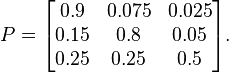
Assuming we are at initial state 'bear' for the probabilities the result is:




Result: [bull, bear, stagant]









[ 0.15  0.8   0.05]
[ 0.2675   0.66375  0.06875]
[ 0.3575   0.56825  0.07425]
[ 0.42555   0.499975  0.074475]
[ 0.47661   0.450515  0.072875]
[ 0.514745   0.4143765  0.0708785]
[ 0.5431466  0.3878267  0.0690267]
[ 0.56426262  0.36825403  0.06748335]
[ 0.5799453   0.35379376  0.06626094]
[ 0.59158507  0.34309614  0.06531879]
[ 0.60022068  0.33517549  0.06460383]
[ 0.60662589  0.3293079   0.06406621]
[ 0.61137604  0.32495981  0.06366415]
[ 0.61489845  0.32173709  0.06336446]
[ 0.61751028  0.31934817  0.06314155]
[ 0.61944687  0.3175772   0.06297594]
[ 0.62088274  0.31626426  0.062853  ]
[ 0.62194736  0.31529086  0.06276178]
[ 0.6227367   0.31456919  0.06269412]
[ 0.62332193  0.31403413  0.06264394]
[ 0.62375584  0.31363743  0.06260672]
[ 0.62407756  0.31334332  0.06257913]
[ 0.62431608  0.31312525  0.06255867]
[ 0.62449293  0.31296357  0.0625435 ]
[ 0.62462404  0.3128437   0.06253225]
[ 0.62472126  0.31275483  0.06252391]
[ 0.62479334  0.31268894  0.06251773]
[ 0.62484677  0.31264008  0.06251314]
[ 0.6248864   0.31260386  0.06250975]
[ 0.62491577  0.312577    0.06250723]
[ 0.62493755  0.31255709  0.06250536]
[ 0.6249537   0.31254233  0.06250397]
[ 0.62496567  0.31253138  0.06250294]
[ 0.62497455  0.31252327  0.06250218]
[ 0.62498113  0.31251725  0.06250162]
[ 0.62498601  0.31251279  0.0625012 ]
[ 0.62498963  0.31250948  0.06250089]
[ 0.62499231  0.31250703  0.06250066]
[ 0.6249943   0.31250521  0.06250049]
[ 0.62499577  0.31250387  0.06250036]
[ 0.62499687  0.31250287  0.06250027]
[ 0.62499768  0.31250212  0.0625002 ]
[ 0.62499828  0.31250158  0.06250015]
[ 0.62499872  0.31250117  0.06250011]
[ 0.62499905  0.31250087  0.06250008]
[ 0.6249993   0.31250064  0.06250006]
[ 0.62499948  0.31250048  0.06250004]
[ 0.62499961  0.31250035  0.06250003]
[ 0.62499971  0.31250026  0.06250002]
[ 0.62499979  0.31250019  0.06250002]
[ 0.62499984  0.31250014  0.06250001]
[ 0.62499988  0.31250011  0.06250001]
[ 0.62499991  0.31250008  0.06250001]
[ 0.62499994  0.31250006  0.06250001]
[ 0.62499995  0.31250004  0.0625    ]
[ 0.62499996  0.31250003  0.0625    ]
[ 0.62499997  0.31250002  0.0625    ]
[ 0.62499998  0.31250002  0.0625    ]
[ 0.62499999  0.31250001  0.0625    ]
[ 0.62499999  0.31250001  0.0625    ]
[ 0.62499999  0.31250001  0.0625    ]
[ 0.62499999  0.31250001  0.0625    ]
[ 0.625   0.3125  0.0625]

AstroML for Creating Histograms in Python

Creating histograms is not that simple as it may seem! There are of course default approaches for creating a histogram, but it is nevertheless better to know what you get instead of just looking at the resulted chart. Besides, we need not only the chart per se, but also the frequency of our data linked to respective bins. It should also be noted while it is useful to customize binning there is no guarantee it yields better result than the automatically binning.

Python offers wide range of possibilities to create histograms. But with this post I would like to introduce AstroML. AstroML (http://www.astroml.org/) is a Python module for machine learning and data mining for astronomy. 

First, let’s present some theoretical background on bin width methods. First, the two most popular rules of thumb for defining bin-width, i.e. Freedman-Diaconis and Scott and second – rules that use fitness functions, i.e. Bayesian blocks and Knuth.

The bin-width (h) and number of bins (W) under Freedman-Diaconis and Scott rules are calculated as follows: 

The other two – Bayesian blocks and Knuth’s rules – are more computationally challenging as they require minimization of a cost function. Astropy (http://astropy.readthedocs.org/en/latest/index.html) gives a brief info: Knuth’s rule chooses a constant bin size which minimizes the error of the histogram’s approximation to the data, while the Bayesian Blocks uses a more flexible method which allows varying bin widths.

Example: I use daily price data for Fondul Proprietatea (ticker: FP), a Bucharest Stock Exchange listed company. My data is stored as csv-file.

!pip install astroML

import pandas as pd

import numpy as np

from astroML.plotting import hist

data=pd.read_csv('FP.csv', delimiter=';')

ret=data/data.shift(1)-1 #calculate simple return

ret= ret['FP'][~np.isnan(ret['FP'])] #remove NaN in the first row of the column (since we calculate returns we get NaN in the first day) and ‘FP’  in this code indicates the name of the column

hist(ret, bins='knuth') #Knuth’s rule

hist(ret, bins='blocks') #Bayesian blocks

hist(ret, bins='freedman') #Freedman-Diaconis

hist(ret, bins='scott') #Scott

We have our return series divided into different number of bins: ranging from 11 bins (Bayesian blocks) to 46 (Knuth’s rule).

Just for the nice math we can create our own code for bins calculation: let’s do something for the Freedman-Diaconis rule:

binwidth=2*(np.percentile(ret,75)-np.percentile(ret,25))*len(ret)**(-1.0/3.0) # bin-width is calculated in accordance with formula above.

bins=np.subtract(ret.max(),ret.min())/binwidth #this is the number of bins

plt.hist(ret.values, bins=np.linspace(min(ret), max(ret), bins))

Or alternatively (with slightly different result):

plt.hist(ret.values, bins=np.arange(ret.min(), ret.max() + binwidth, binwidth))

Markov Chains in Python: a Simple Weather Model

Weather those days is so unstable and behaves strangely for the season. So, for a rainy Friday evening here is an interesting case for Python use.

Markov property is the memoryless property of a stochastic process, namely the property of future states to depend only upon the present state, not the past states. Markov chain is a process that exhibits Markov property.

Using Wikipedia example of a very simple weather model (https://en.wikipedia.org/wiki/Examples_of_Markov_chains#A_very_simple_weather_model), there is 90% probability for a sunny day tomorrow given a sunny day today and 10% probability for a rainy day tomorrow given sunny day today. Also, there is 50% probability for a sunny day tomorrow given a rainy day today and 50% probability for a rainy day tomorrow given a rainy day today. Briefly:

To solve for the weather tomorrow we need two numbers: (1) transition probabilities (as described above) and (2) initial state - what is the weather today (for instance, if today is sunny - we use (1,0), if it is rainy (0,1). Finally, we use matrix multiplication (bear in mind the difference between matrix multiplication and element-wise multiplication) to solve the problem.  The resulted state depends on previous state (changing initial state) and transition probabilities (the transition probabilities matrix remains unchanged).

Next day probability for a sunny day is 90% and probability for a rainy day is 10%. After certain number of predictions, eventually the steady state is reached and the weather prediction for the next day is independent of the initial weather. In our example at some point we reach a probability for a sunny day of 83%. and it barely changes (you can see the result below).

Here is a simple Python implementation of the weather model for a 20-day period: 

import numpy as np

transition=np.array([[0.9, 0.1],[0.5, 0.5]])

initial=np.array([1,0])

for i in range(20):

    n = 0

    counter = 0

    while counter <= n:

        counter+=1

        initial=np.dot(initial,transition)

    print (initial)

Result:

[ 0.9  0.1]

[ 0.86  0.14]

[ 0.844  0.156]

[ 0.8376  0.1624]

[ 0.83504  0.16496]

[ 0.834016  0.165984]

[ 0.8336064  0.1663936]

[ 0.83344256  0.16655744]

[ 0.83337702  0.16662298]

[ 0.83335081  0.16664919]

[ 0.83334032  0.16665968]

[ 0.83333613  0.16666387]

[ 0.83333445  0.16666555]

[ 0.83333378  0.16666622]

[ 0.83333351  0.16666649]

[ 0.8333334  0.1666666]

[ 0.83333336  0.16666664]

[ 0.83333334  0.16666666]

[ 0.83333334  0.16666666]

[ 0.83333334  0.16666666]

Portfolio Risk-Minimizing Weights Solved in Python

In a previous blogpost (Marginal and Component Value-at-Risk: A Python Example http://elenamarinova.blogspot.com/2015/05/marginal-and-component-value-at-risk.html) the Python way for calculating marginal, component and portfolio VaR was introduced. However, it left the portfolio management task a little bit incomplete as the important stage of extracting the risk-minimizing weights of the shares in the portfolio was missing.

Here is again an example of calculating VaR of a simple model portfolio with added a code for extracting weights that minimize the portfolio VaR. A change in the codes introduced in the previous post was made (we worked with annualized numbers in the previous post) to be more precise in the VaR we want, namely 99% confidence interval, 1-day VaR. (Implemented on Python 3.4)

import pandas as pd

import numpy as np

import pandas.io.data as web

import scipy.optimize as scopt

from scipy.stats import norm

Value=1e5 # $100,000

CI=0.99 # set the confidence interval

tickers =['AAPL', 'MSFT', 'YHOO']

numbers=len(tickers)

data=pd.DataFrame()

for share in tickers:

    data[share]=web.DataReader(share, data_source='yahoo', start='2011-01-01', end='2015-06-08')['Adj Close']

data.columns=tickers

ret=data/data.shift(1)-1 # calculate the simple returns

covariances=ret.cov() #gives the covariance of returns

variances=np.diag(covariances) #extracts variances of the individual shares from covariance matrix

volatility=np.sqrt(variances) #gives standard deviation

weights = np.ones(data.columns.size)/data.columns.size

weights

Out: array([ 0.33333333,  0.33333333,  0.33333333])

Pf_variance=np.dot(weights.T,np.dot(ret.cov(),weights)) #Portfolio variance

Pf_volatility=np.sqrt(Pf_variance) #Portfolio standard deviation

USDvariance=np.square(Value)*Pf_variance

USDvolatility=np.sqrt(USDvariance)

covariance_asset_portfolio=np.dot(weights.T,covariances)

covUSD=np.multiply(covariance_asset_portfolio,Value)

beta=np.divide(covariance_asset_portfolio,Pf_variance)

def VaR():

    # this code calculates Portfolio Value-at-risk (Pf_VaR) in USD-terms and Individual Value-at-risk (IndividualVaR) of shares in portfolio. 

    Pf_VaR=norm.ppf(CI)*USDvolatility

    IndividualVaR=np.multiply(volatility,Value*weights)*norm.ppf(CI)

    IndividualVaR = [ '$%.2f' % elem for elem in IndividualVaR ]

    print ('Portfolio VaR: ', '$%0.2f' %Pf_VaR)

    print ('Individual VaR: ',[[tickers[i], IndividualVaR[i]] for i in range (min(len(tickers), len(IndividualVaR)))])

VaR() # call the function

Out: Portfolio VaR:  $2830.87

Individual VaR:  [['AAPL', '$1289.91'], ['MSFT', '$1123.15'], ['YHOO', '$1493.15']]

def marginal_component_VaR():

     # this code calculates Marginal Value-at-risk in USD-terms and Component Value-at-risk of shares in portfolio.

    marginalVaR=np.divide(covUSD,USDvolatility)*norm.ppf(CI)

    componentVaR=np.multiply(weights,beta)*USDvolatility*norm.ppf(CI)

    marginalVaR = [ '%.3f' % elem for elem in marginalVaR ]

    componentVaR=[ '$%.2f' % elem for elem in componentVaR ]

    print ('Marginal VaR:', [[tickers[i], marginalVaR[i]] for i in range (min(len(tickers), len(marginalVaR)))])

    print ('Component VaR: ', [[tickers[i], componentVaR[i]] for i in range (min(len(tickers), len(componentVaR)))])

marginal_component_VaR()# call the function

Out: Marginal VaR: [['AAPL', '0.027'], ['MSFT', '0.023'], ['YHOO', '0.034']]

Component VaR:  [['AAPL', '$908.03'], ['MSFT', '$783.18'], ['YHOO', '$1139.65']]

# Risk-minimizing approach; first, we set the objective function and then we minimize it by changing weights

def VaR(weights):

    return norm.ppf(CI)*np.sqrt(np.square(Value)*(np.dot(weights.T,np.dot(ret.cov(),weights))))

def minVaR(VaR):
    nstocks = data.columns.size
    bounds = [(0.,1.) for i in np.arange(nstocks)] #non-negative weights 
    constraints = ({'type': 'eq',
                        'fun': lambda weights: np.sum(weights) - 1}) #sum of weights to equal 100%
    results = scopt.minimize(VaR, weights,
                                 method='SLSQP',
                                 constraints = constraints,
                                 bounds = bounds)
    result_weights=np.round(results.x, 4)
    result_weights= [ '%.8f' % elem for elem in result_weights ]
    new_VaR=VaR(results['x'])
             
    print ('Optimal VaR: ', new_VaR)
    print ('Optimal Weights: ', [[tickers[i], result_weights[i]] for i in range (len(tickers))])

 minVaR(VaR) # call the function

Out: Optimal VaR:  2756.04924565

Optimal Weights:  [['AAPL', '0.328'], ['MSFT', '0.475'], ['YHOO', '0.197']]

Moving Average Crossover in Python

Developing a successful algorithmic trade strategy is a challenging task, and not just because it is difficult to predict price movements based on past behavior (this is close to what we all have been taught and probably learned in our day-to-day lives). The underlying idea behind algo trading is to exploit market patterns. But market patterns do change, so fast reaction is crucial.

I was trying recently to work on some algo trade codes on Python (Python 2.7) and I ended up for a simple moving average crossover code (15-day moving average and 50-day moving average). The example is for Microsoft shares (ticker: MSFT). Moving average crossover signal is: (i) buy when 15-day moving average crossed above the 50-day moving average and (ii) sell when the 15-day moving average crossed below the 50-day moving average.

Inspired by Aaron Ash’s post “Fun With Python” (http://aaronash.com.au/posts/fun_with_python/) here is what I get:

import pandas as pd
from pandas import *
import StringIO
import urllib
import datetime
import matplotlib.pyplot as plt

%matplotlib inline

def get_data(ticker):

    base_url = 'http://ichart.finance.yahoo.com/table.csv?'

    search_query = 's={}'.format(ticker)

    search_url = '{}{}'.format(base_url, search_query)

    read_url=urllib.urlopen(search_url).read()

    return read_url

# for Python 3.4: read_url=urllib.request.urlopen(search_url).read(); for Python 2.7: read_url=urllib.urlopen(search_url).read()

if __name__ == '__main__':

    ticker = 'MSFT' #select ticker

data=get_data(ticker)

lines = data.split('\n')

lines.reverse()

lines[0] = lines[-1]

cleaned_data = "\n".join(lines[0:-1])

data = read_csv(StringIO.StringIO(cleaned_data))

data.tail() # to see how the data looks like

# calculate the 15-day and 50-day simple moving average (MA)

data['MA_15'] = rolling_mean(data.Close, 15)
data['MA_50'] = rolling_mean(data.Close, 50)
previous_15 = data['MA_15'].shift(1)
previous_50 = data['MA_50'].shift(1)

crossing = (((data['MA_15'] <= data['MA_50']) & (previous_15 >= previous_50))
| ((data['MA_15'] >= data['MA_50']) & (previous_15 <= previous_50)))
crossing_dates = data.loc[crossing, 'Date']
print(crossing_dates) #see where are the crossing points, triggering action

final=DataFrame(data, columns=['Date', 'Close', 'MA_15', 'MA_50'])

final['Date'] = pd.to_datetime(final['Date'])

for_chart=final[final['Date'] >= datetime.date(2013,1,1)]  #to see the results since Jan 1, 2013

# plot the results since Jan 1, 2013

for_chart.plot('Date', 'Close')

for_chart.plot('Date', 'MA_15')
for_chart.plot('Date', 'MA_50')
plt.legend(['Close', 'MA_15', 'MA_50'], loc='upper left')

To see the crossover dates triggers (buy or sell):

crossing_dates=pd.DataFrame(crossing_dates, columns=['Date'])

final=pd.DataFrame(data, columns=['Date', 'Close', 'MA_15', 'MA_50'])

result=crossing_dates.merge(final, on='Date')

result

result['Strategy'] = 0

condition = result['MA_15'] > result['MA_50']

result.loc[condition, 'Strategy'] = 'Buy'

result.loc[~condition, 'Strategy'] = 'Sell'

result

Marginal and Component Value-at-Risk: A Python Example

Value-at-risk (VaR), despite its drawbacks, is a solid basis to understand the risk characteristics of the portfolio. There are many approaches to calculate VaR (historical simulation, variance-covariance, simulation). Marginal VaR is defined as the additional risk that a new position adds to the portfolio. The practical reading of the marginal VaR, as very nicely stated in Quant at risk http://www.quantatrisk.com/2015/01/18/applied-portfolio-value-at-risk-decomposition-1-marginal-and-component-var/ is: the highest the marginal VaR, the exposure to the respective asset should be reduced to lower the portfolio VaR. The component VaR shows the reduction of the portfolio value-at-risk resulting from removal of a position. The sum of component VaR of the shares in the portfolio equals the portfolio diversified VaR, while the sum of the individual VaR presents the undiversified portfolio VaR, assuming perfect correlation between assets in the portfolio.

Also it is worth noting that based on simple mathematics, the equations can be changed, i.e. there are several ways to calculate the component VaR.

We take the following steps in Python to come up with the marginal VaR of a 3-asset portfolio:

(This works for Python 2.7 for Python 3.4 -> change in print statements in the codes. Additionally, to some of the lines some formatting can be applied - for instance returns are not presented in percentages.)

import numpy as np

import pandas as pd

import pandas.io.data as web

from scipy.stats import norm

Value=1e6 # $1,000,000

CI=0.99 # set the confidence interval

tickers =['AAPL', 'MSFT', 'YHOO']

numbers=len(tickers)

data=pd.DataFrame()

for share in tickers:

    data[share]=web.DataReader(share, data_source='yahoo', start='2011-01-01', end='2015-05-15')['Adj Close']

data.columns=tickers

ret=data/data.shift(1)-1 # calculate the simple returns

ret.mean()*252 #annualize the returns

covariances=ret.cov()*252 #gives the annualized covariance of returns

variances=np.diag(covariances) #extracts variances of the individual shares from covariance matrix

volatility=np.sqrt(variances) #gives standard deviation

weights=np.random.random(numbers)

weights/=np.sum(weights) # simulating random percentage of exposure of each share that sum up to 1; if we want to plug in our own weights use: weights=np.array([xx,xx,xx])

Pf_ret=np.sum(ret.mean()*weights)*252 #Portfolio return

Pf_variance=np.dot(weights.T,np.dot(ret.cov()*252,weights)) #Portfolio variance

Pf_volatility=np.sqrt(Pf_variance) #Portfolio standard deviation

USDvariance=np.square(Value)*Pf_variance

USDvolatility=np.sqrt(USDvariance)

covariance_asset_portfolio=np.dot(weights.T,covariances)

covUSD=np.multiply(covariance_asset_portfolio,Value)

beta=np.divide(covariance_asset_portfolio,Pf_variance)

def VaR():

    # this code calculates Portfolio Value-at-risk (Pf_VaR) in USD-terms and Individual Value-at-risk (IndividualVaR) of shares in portfolio.  

    Pf_VaR=norm.ppf(CI)*USDvolatility

    IndividualVaR=np.multiply(volatility,Value*weights)*norm.ppf(CI)

    IndividualVaR = [ '$%.2f' % elem for elem in IndividualVaR ]

    print 'Portfolio VaR: ', '$%0.2f' %Pf_VaR

    print 'Individual VaR: ',[[tickers[i], IndividualVaR[i]] for i in range (min(len(tickers), len(IndividualVaR)))]

VaR() #call the function to get portfolio VaR and Individual VaR in USD-terms

def marginal_component_VaR():

     # this code calculates Marginal Value-at-risk in USD-terms and Component Value-at-risk of shares in portfolio. 

    marginalVaR=np.divide(covUSD,USDvolatility)*norm.ppf(CI)

    componentVaR=np.multiply(weights,beta)*USDvolatility*norm.ppf(CI)

    marginalVaR = [ '%.3f' % elem for elem in marginalVaR ]

    componentVaR=[ '$%.2f' % elem for elem in componentVaR ]

    print 'Marginal VaR:', [[tickers[i], marginalVaR[i]] for i in range (min(len(tickers), len(marginalVaR)))]

    print 'Component VaR: ', [[tickers[i], componentVaR[i]] for i in range (min(len(tickers), len(componentVaR)))]

marginal_component_VaR(): #call the function 

How to Get High Frequency Stock Prices with Python (2): Netfonds Example

Getting high frequency and also real-time stock prices data (for US and Europe stocks in particular) with Python could be very simple indeed! Just use the http://hopey.netfonds.no site. Here is a simple code for generating the url-address (depending on ticker and date), reading and saving the data. Additionally, historical daily high-frequency data is available back for several days (about 15 days). 

The  url- format for the high-frequency data is (the example uses OMV shares, traded on Vienna Stock Exchange): http://hopey.netfonds.no/tradedump.php?date=20150507&paper=E-OMVV.BTSE&csv_format=txt. While for the depth the url-format is http://hopey.netfonds.no/posdump.php?date=20150507&paper=E-OMVV.BTSE&csv_format=txt. However, it seems that depth data is not available for US shares. 

Here is the code and enjoy the data:

import urllib.request

# urllib.request for Python 3.4 and urllib for Python 2.7, respectively change the def get_data(date,ticker,exchange) code below in read_url line

def get_data(date,ticker,exchange):

    base_url = 'http://hopey.netfonds.no/tradedump.php?'

    search_query = 'date={}&paper={}.{}&csv_format=txt'.format(date,ticker,exchange)

    search_url = '{}{}'.format(base_url, search_query)

    read_url=urllib.request.urlopen(search_url).read()

    return read_url

# for Python 3.4: read_url=urllib.request.urlopen(search_url).read(); for Python 2.7: read_url=urllib.urlopen(search_url).read()

if __name__ == '__main__':

    ticker = 'AAPL' # the code-format for US stocks is using directly the ticker, for instance 'AAPL' is Apple, 'MSFT' is Micrrosoft; the format for European shares is 'E-XXXX', for instance 'E-BAYND' - Bayer, 'E-TKAV' -  Telekom Austria, 'E-LLOYL' - Lloyds Banking Group

    date=20150507 # date format is YYYYMMDD

    exchange='O' # 'O' - US shares, 'BTSE' - for European shares

data=get_data(date,ticker,exchange)

with open ("trades.txt", "wb") as f:

    f.write(data)

Generating Correlated Random Numbers: Cholesky Decomposition

When it comes to generate random numbers most of the people see this exercise as a black box. In order to add some colour to this. There are several approaches to generate correlated random numbers, of which two are mainly used, namely Cholesky decomposition and spectral (eigenvalue) decomposition. These types of decomposition are used in copula estimates.

Cholesky decomposition takes the correlation (or covariance) matrix along with randomly generated numbers and correlates them. Cholesky decomposition has two, let’s call it, versions: lower and upper triangular. The Cholesky decomposition can be done in Python via Numpy and SciPy linear algebra (linalg) libraries:

(1) np.linalg.cholesky(A) # using numply linear algebra library and

(2) scipy.linalg.cholesky(A, lower=True) # using SciPy linear algebra library with lower=True indicating we want lower triangular, if we want upper triangular: lower=False. 

I prefer to use the lower triangular matrix. I also prefer working with array instead of matrix.  

Put into practice and using Python, the things look like this (we work with 3 variables):

import numpy as np

from scipy.linalg import cholesky

from scipy.stats import norm

A=np.array([[1,0.1558, 0.2227], [0.1558,1,0.5118], [0.2227,0.5118,1]]) # set the correlation matrix

B= norm.rvs(size=(3, 10000)) # 10,000 simulations to generate 3 random normally distributed variables

Cholesky = cholesky(A, lower=True) # Cholesky decomposition - lower triangular matrix

result= np.dot(Cholesky, B) # generates correlated variables

correlation=np.corrcoef(result) #check the correlation of the simulated variables

By the way, checking if the initial matrix is positive definite is also quite easy on Python:

from scipy.linalg import eigh

eigh(A) # the first array is eigenvalues and the second is eigenvectors

In our example, the correlation matrix is positive definite, meaning that all its eigenvalues are positive.  The eigenvalues of the above correlation matrix are: 0.4832, 0.8903, 1.6265.



Cholesky decomposition can also be used in the opposite case - to uncorrelate variables that are correlated.